

Lineament Extraction from Digital Terrain Derivate Model: A Case Study in the Girón–Santa Isabel Basin, South Ecuador


Abstract
:1. Introduction
- Manual lineament extraction is applied when the main objective is to delineate geological features [17]. It uses image-filtering techniques, band analysis, and transformation, among others. It is performed with visual interpretation and the manual digitization of the lineaments by human operators [18,19].
- Semi-automated lineament extraction is performed by analyzing digital images through an initial automated process (the detection and extraction of the lineaments) and a second phase that corresponds to the interpretation and addition of the detected lineaments. This last step is performed by an operator [20,21] since after extracting the lineaments, manual editing is required to achieve a complete and correct set of linear features [22].
- Automated lineament extraction is performed by analyzing digital images thanks to computer-assisted software. This automated processing includes the development of various algorithms responsible for improving the image, filtering, and detecting edges; it concludes with the extraction of lineaments and delivers the final lineament map in vector format. Some algorithms can be used, such as Hough Transform [23], Segment Tracing Algorithm (STA) [20], Lineament Extraction and Stripe Statistical Analysis (LESSA) [24], Canny Algorithm [25], and Lineament Detection and Analysis (LINDA) [26]. According to [27], the automated algorithms implemented in the extraction of lineaments consider the noise, the threshold, the size, and the orientation of the linear features. The automatic extraction process depends on the efficiency of these algorithms, as well as the content of the information present in the base image [28].
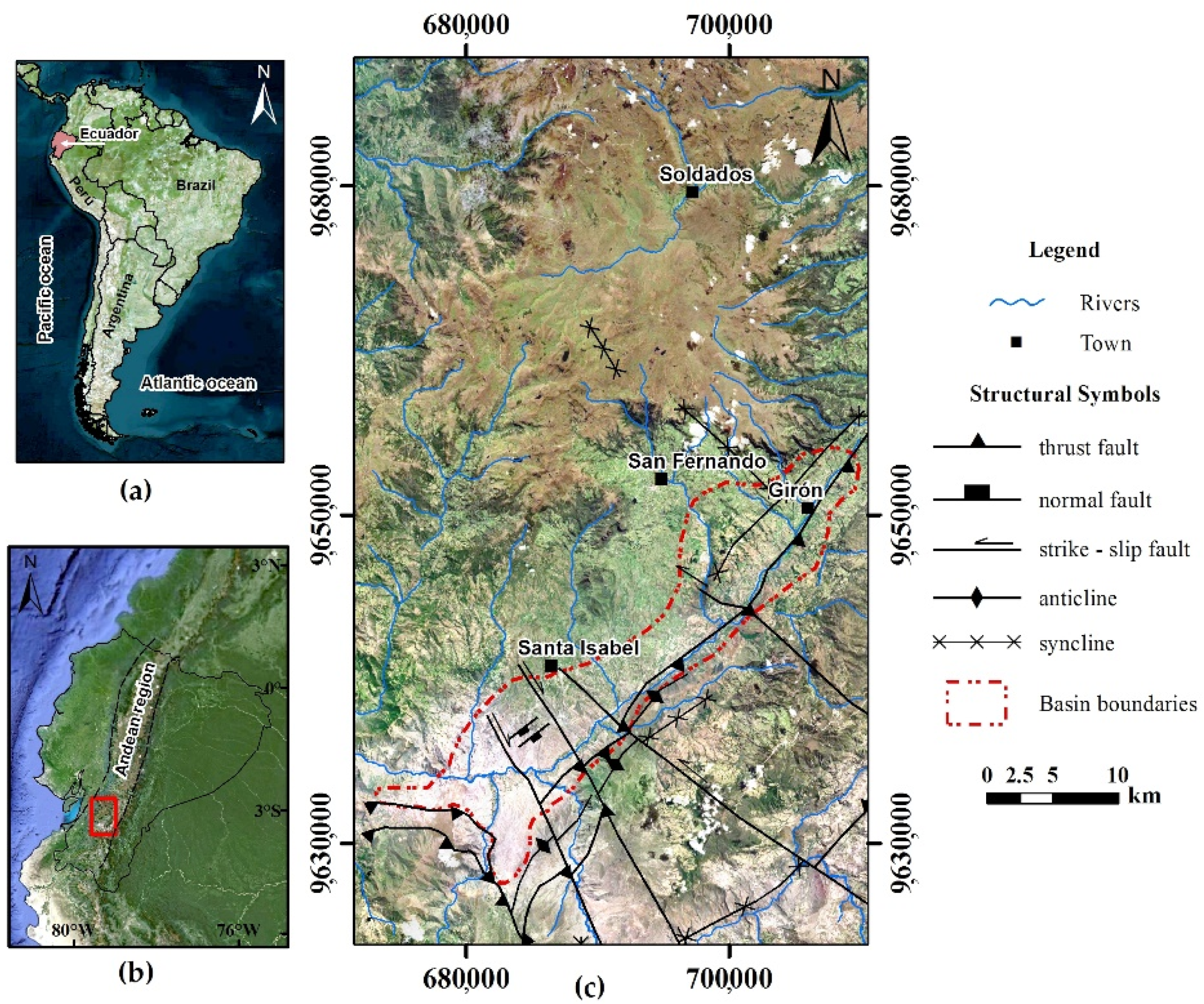
2. Geomorphological and Geological Settings
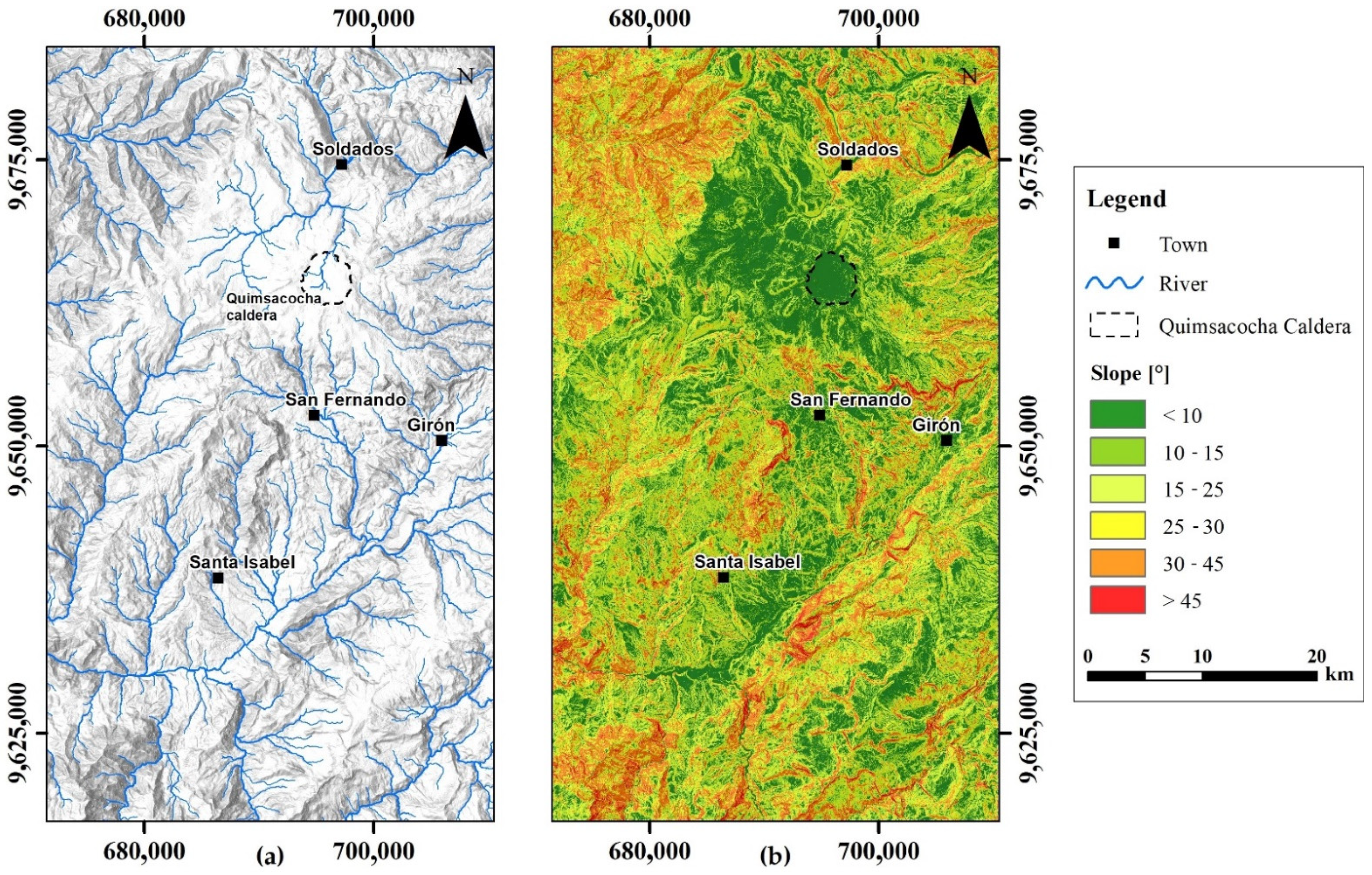
2.1. Geomorphology
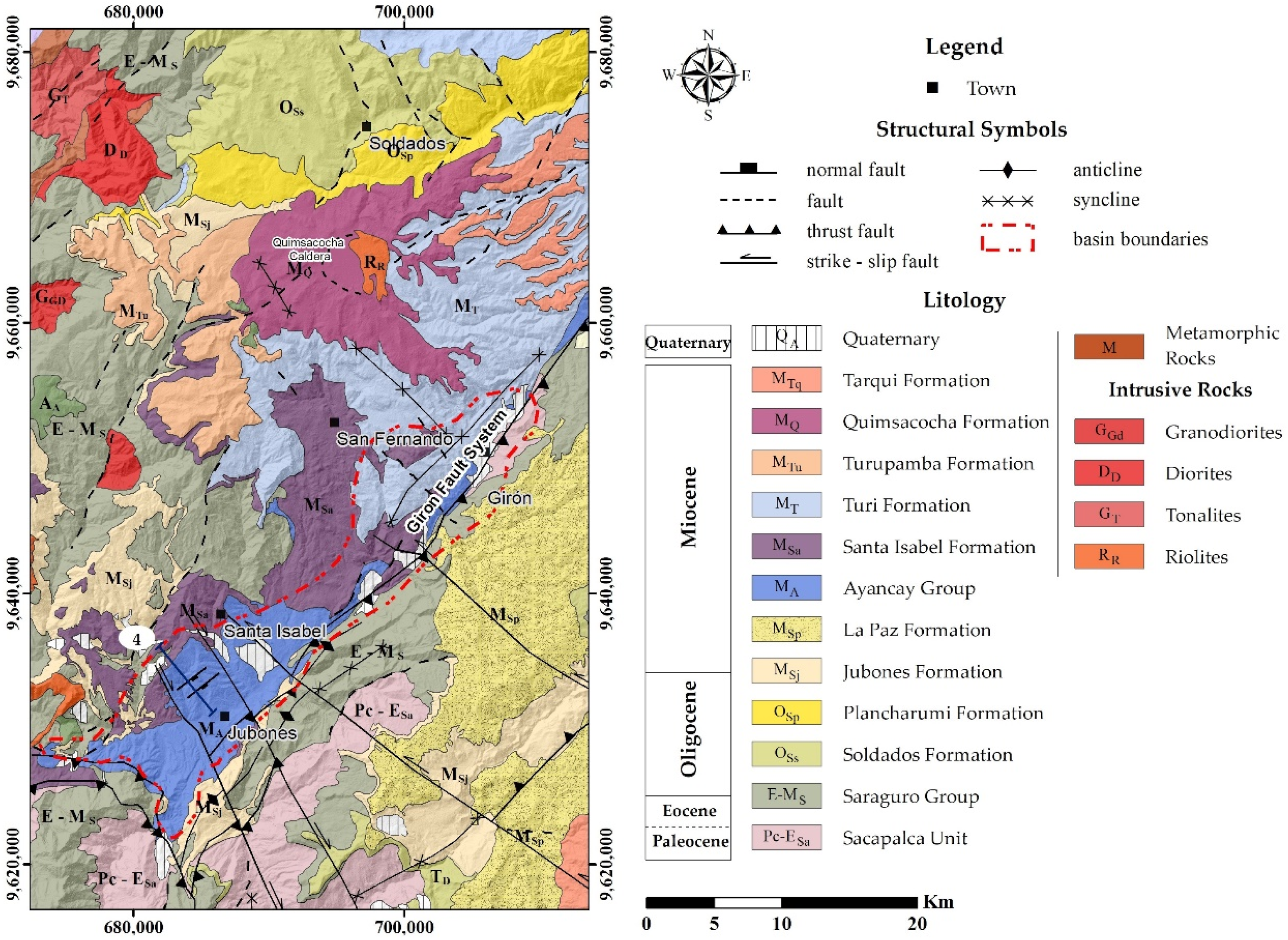
2.2. Geological Setting
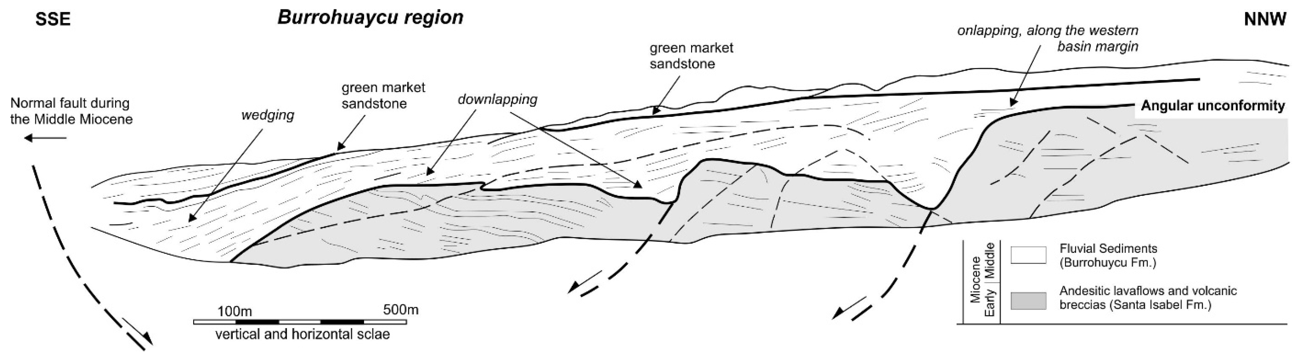
2.2.1. Middle Miocene Extension
2.2.2. Late Miocene—Compression
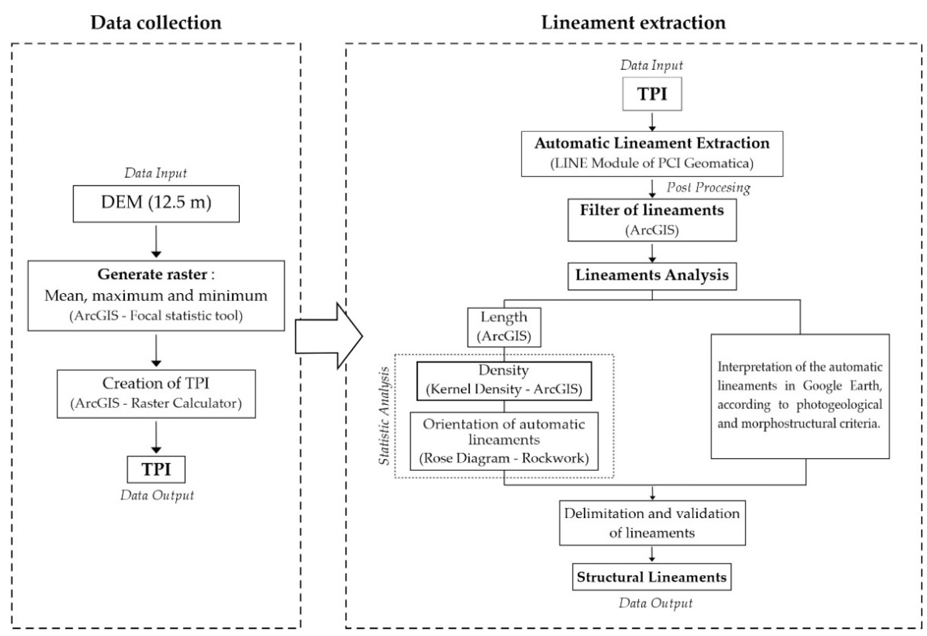
3. Data and Methodology
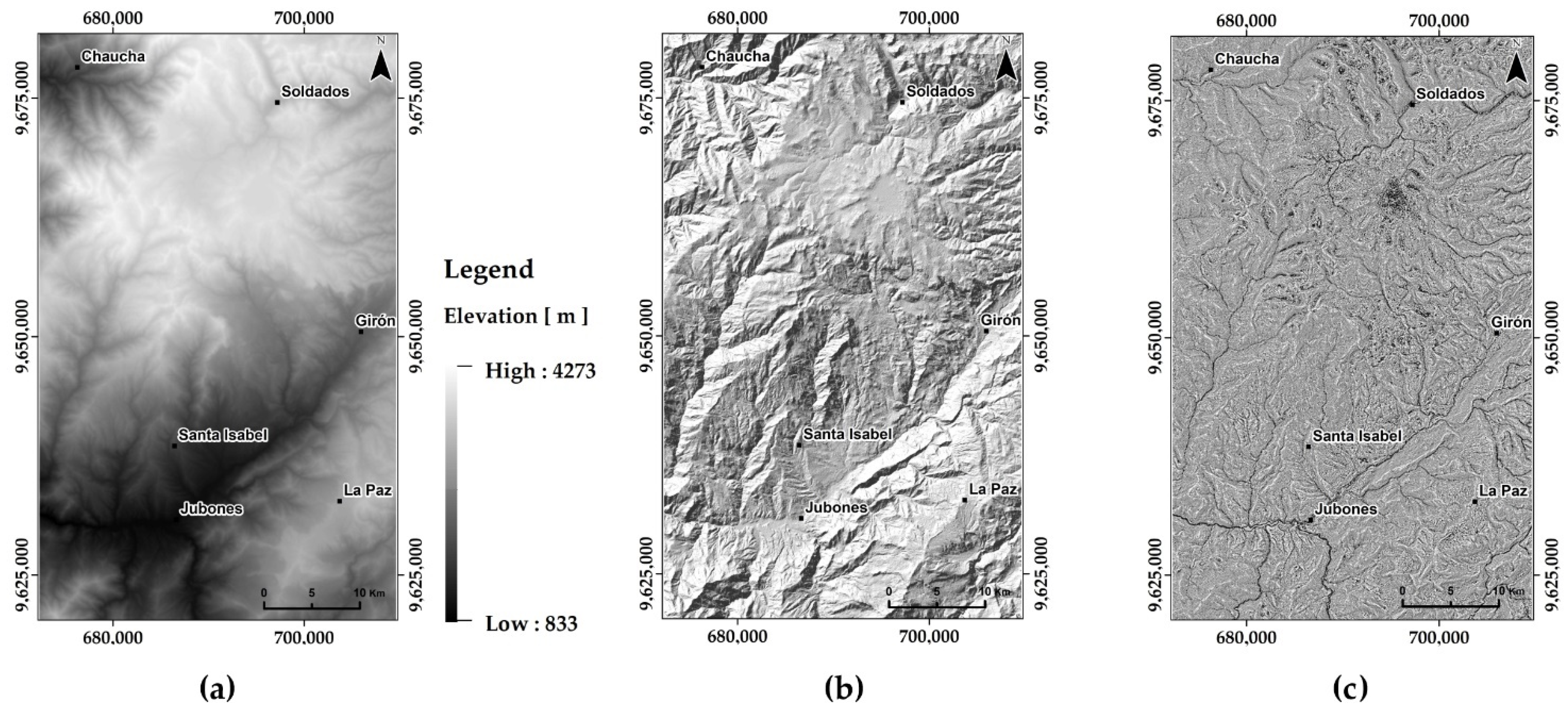
3.1. Data Input
3.2. Processing of Remote Sensing Data
- The RADI represents the smallest level of detail that will be detected in the input image. That is, with this parameter, we establish the minimum length at which linearities will be detected. The value assigned to this parameter depends significantly on the image resolution and the working scale. For our case study, the TPI resolution is 12.5 m, and the working scale is (1:50,000); for this scale, anything smaller than 500 m is not representative [47]. Therefore, 500 m will be considered the minimum detectable distance. This value in pixels corresponds to 40 pixels. Thus, the RADI parameter has a value of 40 pixels.
- GTHR and LTHR influence the number and length of the lines. The GTHR parameter is responsible for edge detection by thresholding the image [46]. This threshold value represents the minimum value (in terms of color) at which changes between two levels or a grayscale with high contrast will be recognized. This value should be in the range of 0 to 255 (Figure 5). The GTHR value is kept at 100, which is the value suggested by the program.
- The value assigned to the LTHR parameter represents the minimum length of the lines extracted by the LINE module. Since the scale of presentation is 1:100,000, anything less than 1000 m is not representative [47]. Therefore, this distance was used as the minimum length to be considered a lineament. Given our image resolution (12.5 m), 1000 m equals 80 pixels.
- FTHR influences accuracy. If high values are assigned to this parameter, longer lines are generated but with a poorer fit. A better fit is obtained with lower values, even though shorter line segments will be obtained. According to [48], values between 3–5 are considered adequate for remote sensing data.
- ATHR is the parameter that influences the joining of lineaments. It represents the maximum angle (in degrees) between segments or vectors to be joined. If the angle between two polyline segments does not exceed the given maximum value, the polyline is joined, resulting in longer lines. On the contrary, if they form an angle greater than the specified maximum, the polyline separates and generates shorter vectors. Hence, a value of 35° is used for this parameter.
- The DTHR parameter sets the separation between the lines. If two segments of a line are close to each other and the separation between them does not exceed the maximum indicated, the segments are linked and form a longer line. For our process, the value of 40 pixels was assigned since it represents the minimum length detected during the analysis.
- The resulting polylines are saved as a vector segment, and the software supports saving them in shapefile format.
3.3. Postprocessing
3.3.1. Filter of Lineaments
3.3.2. Lineament Analysis
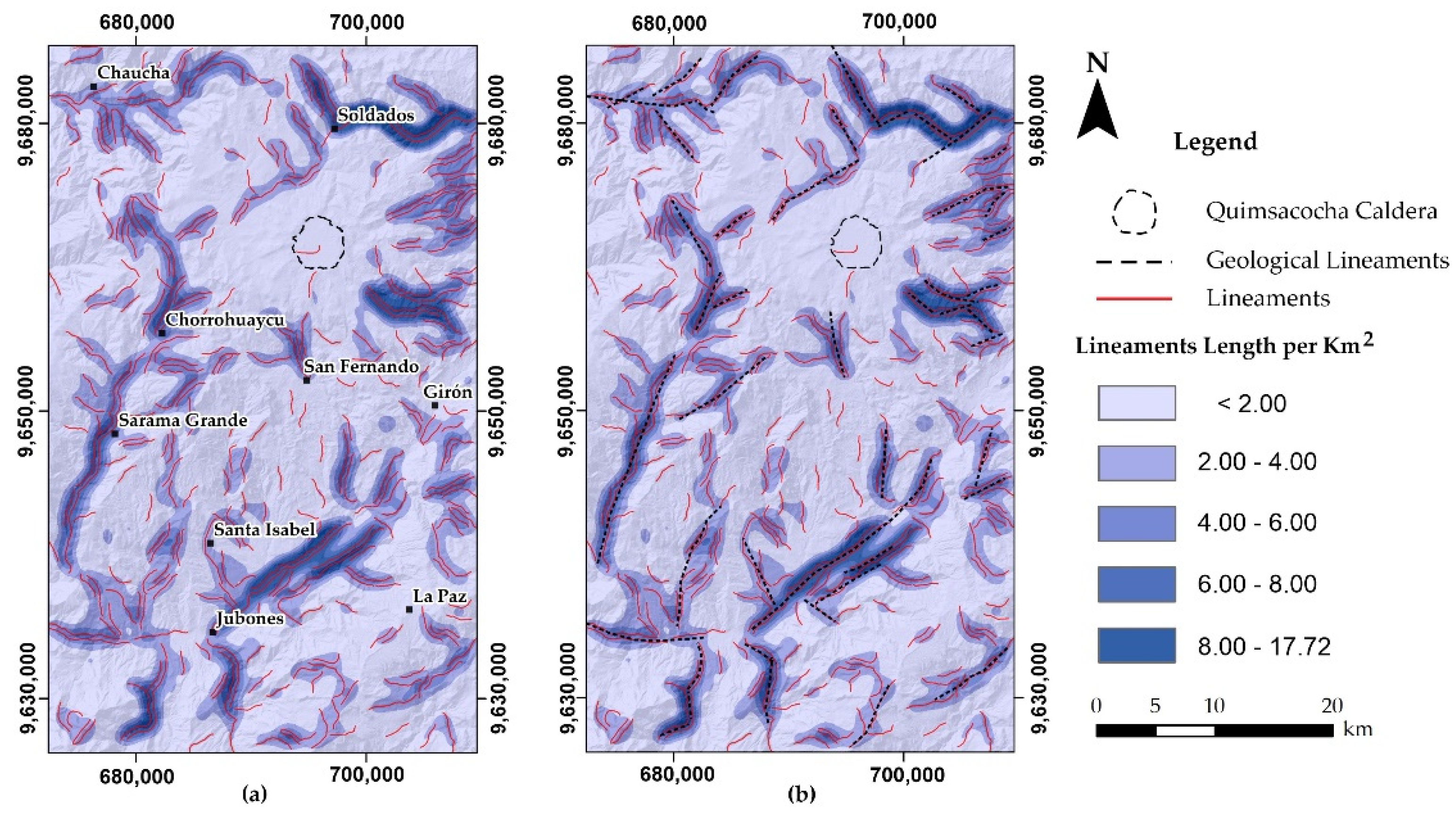
- Line density analysis: Its purpose is to analyze the frequency of lines per unit area (number of lines/km2) [54]. It is obtained by summing the length of available lineaments in a defined grid size (search radius). The lineament density is created with the Kernel density tool [55] of the spatial analyst tool in ArcGIS 10.8.2, with a search radius of 1.5 km according to [48].
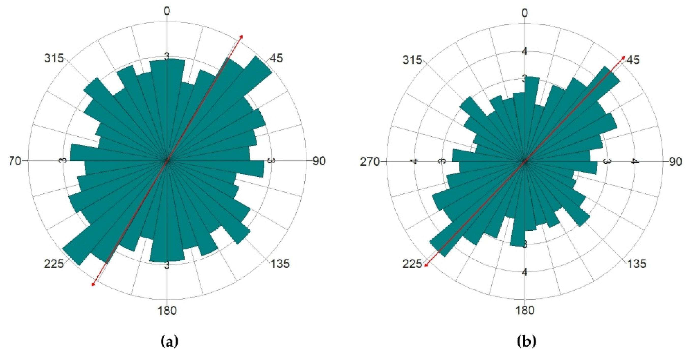
- Lineament orientation: To know the direction of the lineaments in the study area, rose diagrams were generated [56] for the automatically generated lineaments and the lineaments of interest and, finally, to know the predominant orientation of the geological lineaments. These were elaborated in the Rockworks software, version 2016.
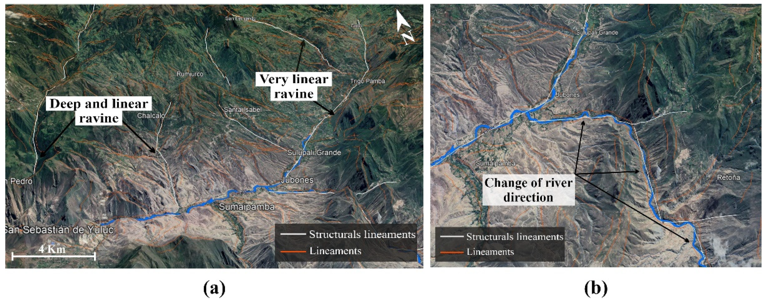
3.4. Delimitation of Geological Lineaments
3.5. Validation
4. Results
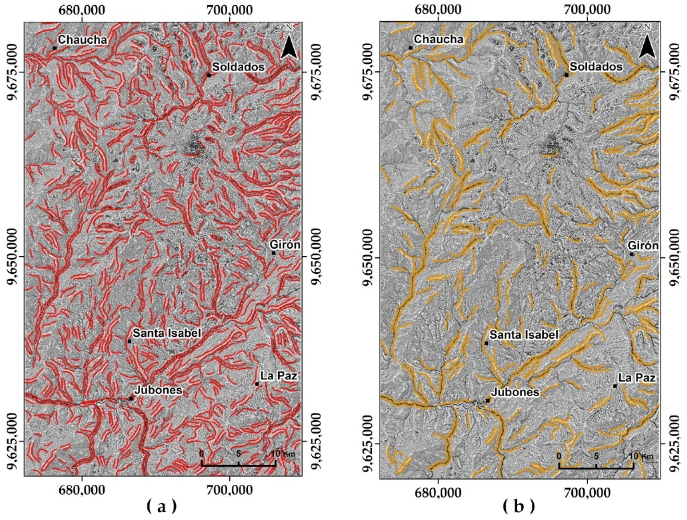
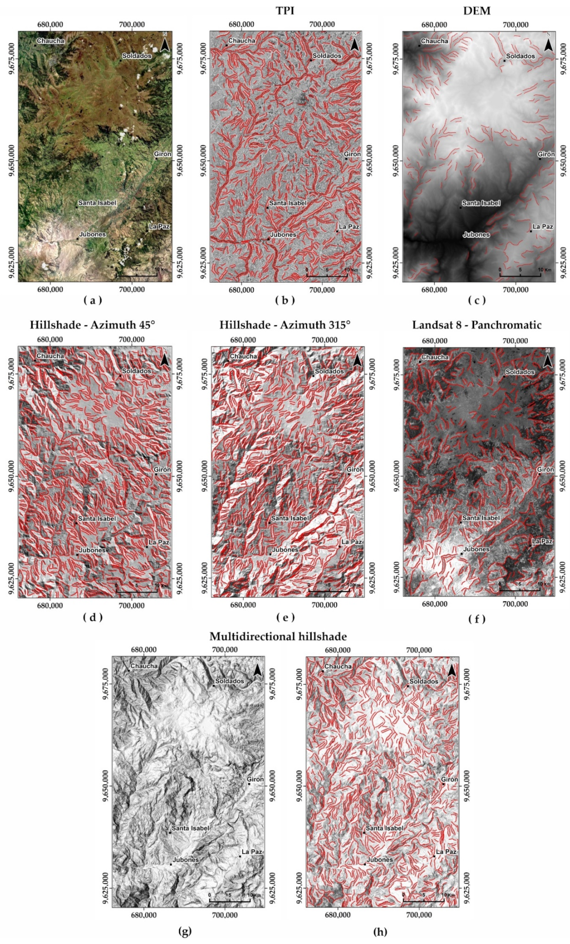
4.1. Comparison
4.2. Postprocessing
4.3. Lineament Density Map
4.4. Orientation of the Lineaments
4.5. Geological Lineaments
5. Discussion
6. Conclusions
Author Contributions
Funding
Acknowledgments
Conflicts of Interest
References
- Hobbs, W.H. Earth Features and Their Meaning; An Introduction to Geology for the Student and the General Reader, 1st ed.; McMillan: New York, NY, USA, 1912; p. 506. [Google Scholar]
- Jordan, G.; Meijninger, B.M.L.; Hinsbergen, D.J.J.; Meulenkamp, J.E.; Dijk, P.M. Extraction of morphotectonic features from DEMs: Development and applications for study areas in Hungary and NW Greece. Int. J. Appl. Earth Obs. Geoinf. 2005, 7, 163–182. [Google Scholar] [CrossRef]
- Tiren, S. Lineament Interpretation. Short Review and Methodology; Progress Report; Swedish Nuclear Fuel and Waste Management Co (SKB), Swedish Hard Rock Laboratory: Stockholm, Sweden, 2010; p. 42. [Google Scholar]
- Hobbs, W.H. Lineaments of the Atlantic Border region. Bull. Geol. Soc. Am. 1904, 15, 483–506. [Google Scholar] [CrossRef]
- Hills, E.S. Elements of Structural Geology, 2nd ed.; John Wiley and Sons: New York, NY, USA, 1972; p. 502. [Google Scholar]
- Ramsay, J.; Huber, M. The Techniques of Modern Structural Geology: Folds and Fractures; Academic Press Inc.: London, UK, 1987; pp. 309–700. [Google Scholar]
- O’leary, D.W.; Friedman, J.D.; Pohn, H.A. Lineament, linear, lineation: Some proposed new standards for old terms: Discussion. Bull. Geol. Soc. Am. 1976, 89, 1463–1469. [Google Scholar] [CrossRef]
- Minár, J.; Sládek, J. Morphological network as an indicator of a morphotectonic field in the central Western Carpathians (Slovakia). Z. Geomorphol. Suppl. Issues 2009, 53, 23–29. [Google Scholar] [CrossRef]
- Ahmadi, H.; Pekkan, E. Fault-Based Geological Lineaments Extraction Using Remote Sensing and GIS—A Review. Geosciences 2021, 11, 183. [Google Scholar] [CrossRef]
- Morelli, M.; Piana, F. Comparison between remote sensed lineaments and geological structures in intensively cultivated hills (Moanferrato and Langhe domains, NW Italy). Int. J. Remote Sen. 2006, 27, 1463–1475. [Google Scholar] [CrossRef]
- Pal, S.K.; Majumdar, T.J.; Bhattacharya, A.K. Extraction of linear and anomalous features using ERS SAR data over Singhbhum Shear Zone, Jharkhand using fast Fourier transform. Int. J. Remote Sens. 2006, 27, 4513–4528. [Google Scholar] [CrossRef]
- Marchionni, D.S.; Cavayas, F. La teledetección por radar como fuente de información litológica y estructural: Análisis espacial de imágenes SAR de RADARSAT-1. Geoacta 2014, 39, 62–89. [Google Scholar]
- Khan, S.D.; Glenn, N. New strike-slip faults and litho units mapped in Chitral (N. Pakistan) using field and ASTER data yield regionally significant results. Int. J. Remote Sens. 2006, 27, 4495–4512. [Google Scholar] [CrossRef]
- Enoh, M.; Okeke, F.; Okeke, U. Automatic lineaments mapping and extraction in relationship to natural hydrocarbon seepage in Ugwueme, South-Eastern Nigeria. Geod. Cartogr. 2021, 47, 34–44. [Google Scholar] [CrossRef]
- Lu, P.F.; An, P. A metric for spatial data layers in favorability mapping for geological events. IEEE Trans. Geosci. Remote Sens. 1999, 37, 1194–1198. [Google Scholar] [CrossRef]
- Guoan, T. Progress of DEM and digital terrain analysis in China. Acta Geogr. Sin. 2014, 69, 1305–1325. [Google Scholar]
- Das, S.; Pardeshi, S.D.; Kulkarni, P.P.; Doke, A. Extraction of lineaments from different azimuth angles using geospatial techniques: A case study of Pravara basin, Maharashtra, India. Arab. J. Geosci. 2018, 11, 160. [Google Scholar] [CrossRef]
- Scheiber, T.; Fredin, O.; Viola, G.; Jarna, A.; Gasser, D.; Łapińska-Viola, R. Manual extraction of bedrock lineaments from high-resolution LiDAR data: Methodological bias and human perception. GFF 2015, 137, 362–372. [Google Scholar] [CrossRef] [Green Version]
- Azman, A.I.; Talib, J.A.; Sokiman, M.S. The integration of remote sensing data for lineament mapping in the semanggol formation, Northwest Peninsular Malaysia. In IOP Conference Series: Earth and Environmental Science; Institute of Physics Publishing: Kuala Lumpur, Malaysia, 2020; Volume 540. [Google Scholar]
- Koike, K.; Nagano, S.; Ohmi, M. Lineament analysis of satellite images using a Segment Tracing Algorithm (STA). Comput. Geosci. 1995, 21, 1091–1104. [Google Scholar] [CrossRef]
- Suzen, M.L.; Toprak, V. Filtering of satellite images in geological lineament analyses: An application to a fault zone in Central Turkey. Int. J. Remote Sens. 1998, 19, 1101–1114. [Google Scholar] [CrossRef]
- Bonetto, S.; Facello, A.; Ferrero, A.M.; Umili, G. A tool for semi-automatic linear feature detection based on DTM. Comput. Geosci. 2015, 75, 1–12. [Google Scholar] [CrossRef]
- Wang, J.; Howarth, P.J. Use of the Hough Transform in Automated Lineament Detection. IEEE Trans. Geosci. Remote Sens. 1990, 28, 561–567. [Google Scholar] [CrossRef]
- Soto-Pinto, C.; Arellano-Baeza, A.; Sánchez, G. A new code for automatic detection and analysis of the lineament patterns for geophysical and geological purposes (ADALGEO). Comput. Geosci. 2013, 57, 93–103. [Google Scholar] [CrossRef]
- Marghany, M.; Hashim, M. Lineament mapping using multispectral remote sensing satellite data. Int. J. Phys. Sci. 2010, 5, 1501–1507. [Google Scholar] [CrossRef]
- Masoud, A.; Koike, K. Applicability of computer-aided comprehensive tool (LINDA: Lineament Detection and Analysis) and shaded digital elevation model for characterizing and interpreting morphotectonic features from lineaments. Comput. Geosci. 2017, 106, 89–100. [Google Scholar] [CrossRef]
- Joshi, A.K. Automatic detection of lineaments from Landsat data. Dig. Int. Geosci. Remote Sens. Symp. 1989, 1, 85–88. [Google Scholar]
- Al-Dossary, S.; Marfurt, K.J. Lineament-preserving filtering. Geophysics 2007, 72, P1–P8. [Google Scholar] [CrossRef]
- Abdullah, A.; Nasser, S.; Ghaleeb, A. Landsat ETM-7 for Lineament Mapping using Automatic Extraction Technique in the SW part of Taiz area, Yemen. Glob. J. Hum. Soc. Sci. Res. 2013, 13, 35–37. [Google Scholar]
- Podwysocki, M.; Moik, J.; Shoup, W. Quantification of geological lineaments by manual and machine processing technique. In NASA Earth Resources Survey Symposium; NASA: Houston, TX, USA, 1975; pp. 885–903. [Google Scholar]
- Parsons, A.J.; Yearley, R.J. An analysis of geologic lineaments seen on LANDSAT MSS imagery. Int. J. Remote Sens. 1986, 7, 1773–1782. [Google Scholar] [CrossRef]
- Divi, R.S.; Zakir, F.A. Delineation of Tectonic Features Utilizing Satellite Remote Sensing Data: I-The Southern-Half of the Arabian Shield. Gondwana Res. 2001, 4, 159–161. [Google Scholar] [CrossRef]
- Das, D.P.; Chakraborty, D.K.; Sarkar, K. Significance of the regional lineament tectonics in the evolution of the Pranhita-Godavari sedimentary basin interpreted from the satellite data. J. Asian Earth Sci. 2003, 21, 553–556. [Google Scholar] [CrossRef]
- Pour, A.B.; Hashim, M. Structural mapping using PALSAR data in the Central Gold Belt, Peninsular Malaysia. Ore Geol. Rev. 2015, 64, 13–22. [Google Scholar] [CrossRef] [Green Version]
- Scheiber, T.; Viola, G. Complex bedrock fracture patterns: A multipronged approach to resolve their evolution in space and time. Tectonics 2018, 37, 1030–1062. [Google Scholar] [CrossRef]
- Abdelkareem, M.; Hamimi, Z.; El-Bialy, M.Z.; Khamis, H.; Abdel Wahed, S.A. Integration of remote-sensing data for mapping lithological and structural features in the Esh El-Mallaha area, west Gulf of Suez, Egypt. Arab. J. Geosci. 2021, 14, 497. [Google Scholar] [CrossRef]
- Prasad, A.D.; Jain, K.; Gairola, A. Mapping of lineaments and knowledge base preparation using geomatics techniques for part of the Godavari and Tapi basins, India: A case study. Int. J. Comput. Appl. 2013, 70, 9. [Google Scholar]
- Weiss, A. Topographic position, and landforms analysis. In Proceedings of the Poster Presentation, ESRI User Conference, San Diego, CA, USA, 9–13 July 2001; p. 200. [Google Scholar]
- Pratt, E.; Figueroa, J.; Flores, B. Informe N° 1, proyecto de desarrollo minero y control ambiental, programa de información cartográfica y geológica: Mapa escala 1: 200.000. In Geology of the Cordillera Occidental of Ecuador between 3° S and 4° S; CODIGEM -BGS: Quito, Ecuador, 1997; p. 58. [Google Scholar]
- Flor, A.; Avilés, H.; Villalta, M.; Murillo, I.; Larreta, E.; Mulas, M. Geotechnical and structural characterization of the Ignimbritas of the Saraguro group in the sector of Santa Isabel-Pucará, Ecuador. In Proceedings of the 17th LACCEI International Multi-Conference for Engineering, Education, and Technology, Montego Bay, Jamaica, 24–26 June 2019. [Google Scholar]
- Hungerbühler, D. Neogene Basins in the Andes of Southern Ecuador: Evolution, Deformation, and Regional Tectonic Implications. Ph.D. Thesis, ETH Zurich, Zurich, Switzerland, 1997. [Google Scholar]
- Siravo, G.; Speranza, F.; Mulas, M.; Costanzo-Alvarez, V. Significance of northern Andes terrane extrusion and genesis of the interandean valley: Paleomagnetic evidence from the “Ecuadorian orocline”. Tectonics 2021, 40, e2020TC006684. [Google Scholar] [CrossRef]
- PALSAR_Radiometric_Terrain_Corrected_high_res; Includes Material © JAXA/METI 2007. Accessed through ASF DAAC 04 Julio 2020. Available online: https://doi.org/10.5067/Z97HFCNKR6VA (accessed on 16 August 2021).
- PCI Geomatics. Geomatica Exploration and Geological Applications; PCI Geomatics: Markham, ON, Canada, 2018. [Google Scholar]
- PCI Geomatics. Geomatica Training Guide; Geomatica, I Course Guide; PCI Geomatics: Markham, ON, Canada, 2018. [Google Scholar]
- PCI Geomatics. CATALYST: LINE. Available online: https://catalyst.earth/catalyst-system-files/help/references/pciFunction_r/easi/E_line.html (accessed on 12 February 2022).
- Chuvieco, E. Fundamentos de Teledetección Espacial, 1st ed.; RIALP, S.A.: Madrid, Spain, 1996. [Google Scholar]
- Hashim, M.; Ahmad, S.; Johari, M.A.M.; Pour, A.B. Automatic lineament extraction in a heavily vegetated region using Landsat Enhanced Thematic Mapper (ETM+) imagery. Adv. Space Res. 2013, 51, 874–890. [Google Scholar] [CrossRef]
- El-Sawy, K.; Ibrahim, A.M.; El-Bastawesy, M.A.; El-Saud, W.A. Automated, manual lineaments extraction and geospatial analysis for Cairo-Suez district (Northeastern Cairo-Egypt), using remote sensing and GIS. Int. J. Innov. Sci. Eng. Technol. 2016, 3, 491–500. [Google Scholar]
- Abdullah, A.; Akhir, J.M.; Abdullah, I. The Extraction of Lineaments Using Slope Image Derived from Digital Elevation Model: Case Study: Sungai Lembing—Maran Area, Malaysia. J. Appl. Sci. Res. 2010, 6, 1745–1751. [Google Scholar]
- Abdullah, A.; Akhir, J.M.; Abdullah, I. Automatic Mapping of Lineaments Using Shaded Relief Images Derived from Digital Elevation Model (DEMs) in the Maran-Sungai Lembing Area, Malaysia. Electron. J. Geotech. Eng. 2010, 15, 949–957. [Google Scholar]
- Salichtchev, K.A. Cartografía; Editorial Pueblo y Educación: La Habana, Cuba, 1979; p. 182. [Google Scholar]
- Vink, A.P.A. Land Use in Advancing Agriculture; Springer: Berlin, Germany; New York, NY, USA, 1975; p. 394. [Google Scholar]
- Greenbaum, D. Revisión de aplicaciones de sensores remotos para la exploración de aguas subterráneas en sótanos y regolito. Br. Geol. Surv. Rep. OD 1985, 85, 36. [Google Scholar]
- Terrell, R.G.; Scott, D.W. Variable kernel density estimation. Ann. Stat. 1992, 20, 1236–1265. [Google Scholar] [CrossRef]
- Chandrasekhar, P.; Martha, T.R.; Venkateswarlu, N.; Subramanian, S.K.; Kamaraju, M. Regional geological studies over parts of Deccan Syneclise using remote sensing and geophysical data for understanding hydrocarbon prospects. Curr. Sci. 2011, 100, 95–99. [Google Scholar]
- Masoud, A.A.; Koike, K. Autodetection, and integration of tectonically significant lineaments from SRTM DEM and remotely sensed geophysical data. ISPRS J. Photogram. Remote Sens. 2011, 66, 818–832. [Google Scholar] [CrossRef]
- Mandeng, E.; Bidjeck, L.; Wambo, J.; Tak, A.; Betsi, T.B.; Ipan, A.S.; Dieudonné, L. Lithologic and structural mapping of the Abiete –Toko gold district in southern Cameroon, using Landsat 7 ETM+/SRTM. Comptes Rendus Geosci. 2018, 350, 130–140. [Google Scholar] [CrossRef]
- García, A.; Zamorano, J.J.; López-Miguel, C.; Galván-García, A.; Carlos-Valerio, V.; Ortega, R.; Macías, J.L. El arreglo morfoestructural de la Sierra de Las Cruces, México central. Rev. Mex. Cienc. Geológicas 2008, 25, 158–178. [Google Scholar]
- Raj, N.; Prabhakaran, A.; Muthukrishnan, A. Extraction and analysis of geological lineaments of Kolli hills, Tamil Nadu: A study using remote sensing and GIS. Arab. J. Geosci. 2017, 10, 195. [Google Scholar] [CrossRef]


| Parameters | Default Values | Suggested Values |
|---|---|---|
| RADI | 10 | 40 |
| GTHR | 100 | * 100 |
| LTHR | 30 | 80 |
| FTHR | 3 | 3 |
| ATHR | 30 | 35 |
| DTHR | 20 | 40 |
| TPI | DEM | Hillshade 45° | Hillshade 315° | Multidirectional Hillshade | Landsat 8—Panchromatic | |
|---|---|---|---|---|---|---|
| No. of lineaments | 1055 | 271 | 1261 | 1297 | 1213 | 653 |
| Max. length (km) | 14.23 | 6.53 | 8.35 | 11.78 | 9.99 | 10.23 |
| Min. length (km) | 1.00 | 1.00 | 1.00 | 1.00 | 1.00 | 1.20 |
| Median length (km) | 1.56 | 1.63 | 1.63 | 1.57 | 1.52 | 1.75 |
| Mean length (km) | 1.94 | 2.01 | 1.95 | 1.92 | 1.77 | 2.04 |
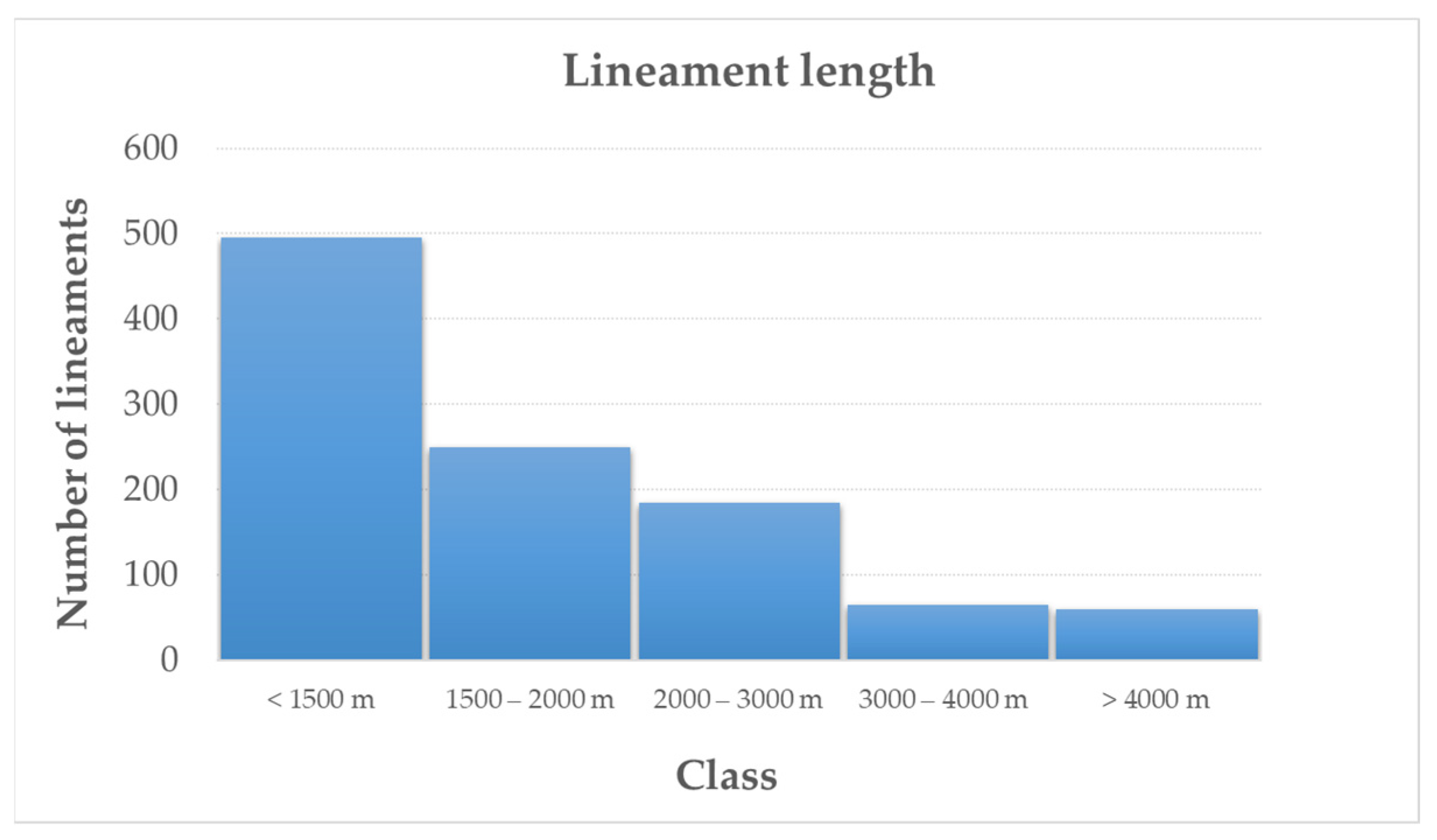
| Lineament Length Class | Range | Number of Lineaments | |
|---|---|---|---|
| (In nos.) | (in %) | ||
| Very short | <1500 m | 496 | 47.01 |
| Short | 1500–2000 m | 249 | 23.60 |
| Medium | 2000–3000 m | 185 | 17.54 |
| Long | 3000–4000 m | 65 | 6.16 |
| Very long | >4000 m | 60 | 5.69 |
| Total | 1055 | 100.00 | |
| Density Class | Density Range (km/km2) | Area | |
|---|---|---|---|
| (in km2) | (in %) | ||
| Very low | <2 | 1479.65 | 64.16 |
| Low | 2–4 | 499.91 | 21.67 |
| Moderate | 4–6 | 199.74 | 8.66 |
| High | 6–8 | 68.45 | 2.97 |
| Very high | >8 | 58.60 | 2.54 |
| Total | 2306.36 | 100.00 | |
Publisher’s Note: MDPI stays neutral with regard to jurisdictional claims in published maps and institutional affiliations. |
© 2022 by the authors. Licensee MDPI, Basel, Switzerland. This article is an open access article distributed under the terms and conditions of the Creative Commons Attribution (CC BY) license (https://creativecommons.org/licenses/by/4.0/).
Share and Cite
Villalta Echeverria, M.D.P.; Viña Ortega, A.G.; Larreta, E.; Romero Crespo, P.; Mulas, M. Lineament Extraction from Digital Terrain Derivate Model: A Case Study in the Girón–Santa Isabel Basin, South Ecuador. Remote Sens. 2022, 14, 5400. https://doi.org/10.3390/rs14215400
Villalta Echeverria MDP, Viña Ortega AG, Larreta E, Romero Crespo P, Mulas M. Lineament Extraction from Digital Terrain Derivate Model: A Case Study in the Girón–Santa Isabel Basin, South Ecuador. Remote Sensing. 2022; 14(21):5400. https://doi.org/10.3390/rs14215400
Chicago/Turabian StyleVillalta Echeverria, Michelle Del Pilar, Ana Gabriela Viña Ortega, Erwin Larreta, Paola Romero Crespo, and Maurizio Mulas. 2022. "Lineament Extraction from Digital Terrain Derivate Model: A Case Study in the Girón–Santa Isabel Basin, South Ecuador" Remote Sensing 14, no. 21: 5400. https://doi.org/10.3390/rs14215400